Climate change at specific measuring stations
The GeoSphere Austria climate monitoring portal contains many interesting statistics, including temperature increases at selected stations compared to previous periods. The aim of this showcase is to move beyond these predefined locations and expand the data to any measuring station in Austria.
Average temperature of a climate normal period (Part 1 – Calculation of monthly averages)
In stages 1 and 2 of this showcase, the mean temperature for an arbitrary GeoSphere Austria measuring station is to be calculated. The Bruck/Mur station in Styria is chosen randomly as an example. The calculation method for such a climatological mean is prescribed by the WMO (World Meteorological Organization).
Data
For the analysis monthly data is required. The parameter "t - monthly mean air temperature 2 m above the ground" is downloaded for the period January 1961 to December 2020. The time frame covers a 60-year span, which includes two complete climate normal periods, typically 30 years each. Since the location of the Bruck/Mur station has been modified twice over time, data from all three available stations must be obtained.
Methods
Monthly mean temperatures for the climate normal periods, i.e. 1961 to 1990 and 1991 to 2020, have to be derived. This means that the monthly values are averaged sepeartely for each month in both timeframes.
Results
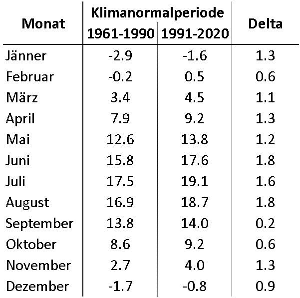
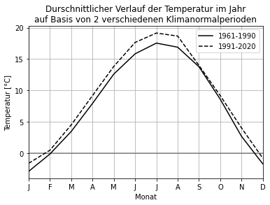
The resulting averages are shown in Table 1.1. Additionally, the difference between the climate normal period of 1961 to 1990 and that of 1991 to 2020 was calculated for each month. It is noticeable that the average temperature increased for all months. A more detailed analysis reveals that the strongest temperature increase occurred in the summer months (June to August), averaging 1.7 °C. This increase was more than twice as large as that in autumn (September to November, 0.7 °C).
Please note the difference of 0.6 °C for February instead of 0.7 °C. This discrepancy arises from rounding subsequently to the calculation.
Appendix / Images
Average Temperature of a Climate Normal Period (Part 2 – Determining the Average Temperature)
Since most of the preliminary work was completed in Step 1, Step 2 can now proceed directly to calculating the average annual temperature of the climate normal periods.
Step 2 – Calculating Annual Average Temperatures
This step, starting with the monthly averages calculated in Step 1, is straightforward and simply involves averaging these twelve values per climate normal period. As in Step 1, this calculation can be performed using a spreadsheet program like Microsoft Excel, or with programming languages such as Python or R.
Results
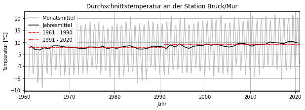
The average temperature for the climate normal period from 1961 to 1990 is 7.9 °C, and for that period from 1991 to 2020, it is 9.0 °C. This corresponds to an increase of 1.1 °C. Monthly and annual means as well as the annual average derived for the climate normal periods are illustrated in Figure 2.1. This figure was created using the Python 3 programming language.
Due to the strong seasonal fluctuations in the monthly data, the change in annual temperature appears less pronounced. The coldest year on average was 1963 with approximately 6.8 °C. The warmest year at the Bruck/Mur station was 2019 with an average of 10.4 °C.
Appendix / Images
Calculation of a Linear Trend
Although the comparison of the climate normal periods evaluated in step 1 and 2 already indicates an increase in mean air temperature, a linear regression will be calculated to illustrate this increase. For this purpose, the same dataset used for the previous calculation of the climate normal periods will be used.
Linear Regression
Linear regression is a simple statistical tool for estimating trends in a series of measurements. It represents a straight line that can be fitted to the available data featuring the smallest possible deviation from all data points when considered together. The method for deriving such a regression line must be consulted in mathematical literature, as the scope of this showcase is insufficient.
Linear regressions are not exclusively used in climatology and meteorology. Depending on the application, careful interpretation is essential. In particular, in the context of this analysis, it is not permissible to extrapolate from the linear regression of the annual mean temperature between 1961 and 2020 at the Bruck/Mur weather station to years before or after this period. Such information is calculated in climatology using specially developed models that are significantly more complex than linear regression.
Results
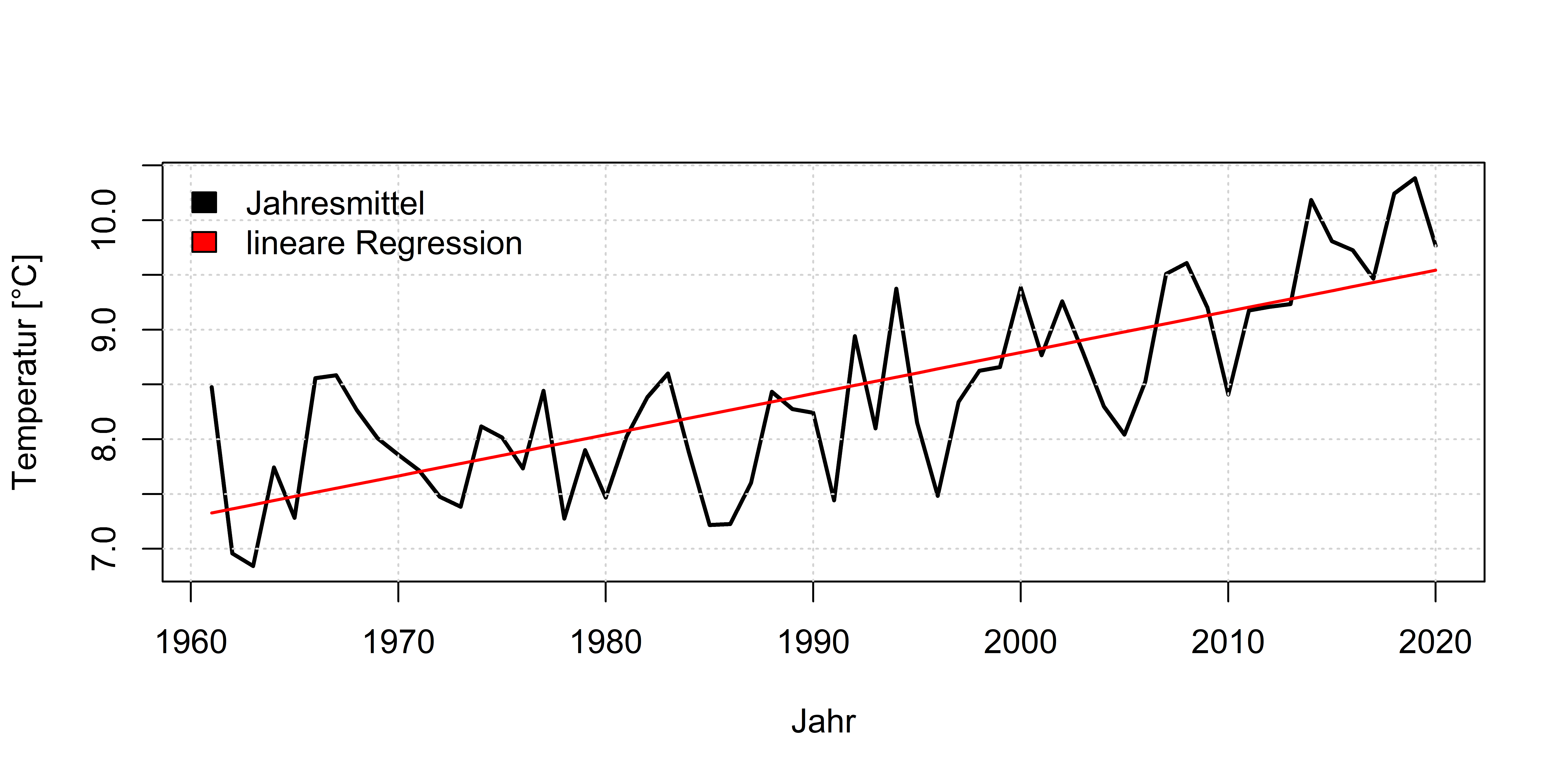
Figure 3.1 shows the result of the linear regression. Unlike Figure 2.1 in step 2, the monthly averages were omitted because they would significantly expand the temperature range on the y-axis, obscuring the increase.
The gradient of the line shown in the upper left corner of the plot indicates that the average annual temperature at the measuring station increased by approximately 0.04 °C per year between 1961 and 2020. Extrapolated over 60 years, this equates to an increase of 2.4 °C. As previously mentioned, it is not permissible to draw conclusions about the period before 1961 or after 2020 based on this trend.
This linear regression was derived and illustrated using Python 3. The analyses shown can be replicated with any other station. The only requirement is the length of the measurement series.
Appendix / Images
Datasets
Dieser Datensatz beinhaltet Monatswerte einer Vielzahl meteorologischer bzw. klimatologischer Parameter. Für alle Klima-Beobachtungstermine ist der Monatsmittelwert der entsprechenden Größen angegeben. Die drei Klima-Beobachtungstermine (I, II,...
Temperature, Humidity, Radiation, Wind, Precipitation, Cloud cover, Pressure, Snow, Sunshine, Visibility, Observed weather phenomena, Thunderstorm
